Forward-Backward Algorithms

This continues from my last post about Hidden Markov models. This includes a review of the forward algorithm, the backward algorithm, and the Baum-Welch algorithm.

The Baum-Welch algorithm allows for the training of a model from a set of observed sequences. The forward-backward algorithms, and their relationship are the foundations of the Baum-Welch algorithm, so to understand the Baum-Welch algorithm we must first have a solid understanding of those concepts.

Notation Used:

Here are the variables used to represent different model parameters, (sorry in advance for any inconsistency):

\[\lambda = \{A, B, \pi\}\] where:

• A is the transition probability matrix where \(a_{ij}\) is the probability of transitioning from state i to j.
• B is the emission probabilitiy matrix where \(b_{j}{k}\) is the probability of observing symbol \(v_{k}\) in state j
• \(\pi\) is the matrix of initial state probabilities, where \(\pi_{i}\) is the probability that state i is the initial state
• \(X=\{x_{1},x_{2},x_{3},…,x_{t}\}\) is a sequence of observed symbols
• \(S=\{s_{1},s_{2},s_{3},…,s_{t}\}\) is a sequence of hidden states
• \(P(X_{t}=v_{k} \vert S_{t} = i)\) is the probability of observing symbol \(v_{k}\) in state i at time t.

Review: Forward Algorithm:

The Forward Probability is the probability of seeing the observations \(x_{1}, x_{2},…,x_{t}\) and being in state i at time t, given a model \(\lambda = \{A, B, \pi\}\).

It uses the computed probability at the current time step to derive the probability of being in a particular hidden state at the next time step.

The forward algorithm calculates this forward probability for all hidden states.

This is found recursively: \[\alpha_{i}(1) = \pi_{i}b_{i}(x_{1})\] \[\alpha_{i}(t+1) = b_{i}(x_{t+1})\sum_{j=1}^N \alpha_{j}(t)a_{ji}\]

where:

• \(\alpha_{i}(t)\) is the probability of being in state i at time t. This is the value that is returned.
• \(\pi_{i}\) is the probability that the initial state is i
• \(b_{i}(x_{t})\) is the probability of seeing symbol \(x_{t}\) in state i
• \(a_{ij}\) is the probability of being in state i given the previous state was state j

(See the post on Hidden Markov Models for more details, and an example)

Backwards Algorithm:

While the forwards algorithm is more intuitive, as it follows the flow of “time”, relating the current state to past observations, backwards probability moves backward through “time” from the end of the sequence to time t, relating the present state to future observations.

Backwards probability is the probability of starting in state \(i\) at time \(t\) and generating the rest of the observation sequence \(x_{t+1}, x_{t+2},…,x_{T}\):

\[\beta_{i}(t) = P(x_{t+1}, x_{t+2}, …. x_{T} \vert s_{t} = i)\]

To compute this probability we use the backwards algorithm. The algorithm starts at time T (the end) and then works backwards throught the sequence from observation symbol \(x_{T}\) down to \(x_{t+1}\).

The initial probabilities of being in state \(i\) at time T, and not observing anything else is 1, because we have reached the end the sequence, so there is no more output.

We write this as:

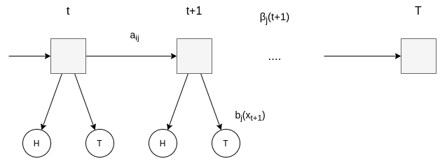
\[\beta_{i}(T) = P(\emptyset \vert s_{T} = i) = 1\] \[\beta_{i}(t) = \sum_{j=1}^N \beta_{j}(t+1)a_{ij}b_{j}(x_{t+1})\] where:

• i is referring to the state i
• T is the last timestep in the sequence, which is equal to the length of the sequence
• \(a_{ij}\) is the probability of transitioning from state i to j
• \(b_{j}(x_{t+1})\) is the probability of observing the symbol \(x_{t+1}\) in state j at time t+1

This can be visualized as (the squares are the hidden states, and the circles the observation symbols)

Back to the fair-casino example

(See previous post for problem details)

If we have a sequence ending in \(X=\{…, H, T, H\}\), we can calculate our backwards probability as follows:

We start at the time T: \[\beta_{F}(T) = 1\] \[\beta_{B}(T) = 1\]

For the recursive step, to calculate the backwards probability for a single hidden state (for example: F - the coin is fair), we do:

\[\beta_{F}(T-1) = \sum_{j=1}^N \beta_{j}(t+1)a_{Fj}b_{j}(x_{t+1}=T)\] \[ = \beta_{F}(t+1)a_{FF}b_{F}(H) + \beta_{B}(t+1)a_{FB}b_{B}(H)\] \[ = (1)(0.9)(0.5) + (1)(0.1)(0.75) = 0.45 + 0.075 = 0.525 \]

Since at each step we would need to calculate the backwards probability for both states, (both fair and biased coins), it would be great if we could do it for both at once.

Using matrices we can do both states in one calculation:

\[\beta(T) = \begin{bmatrix}1 && 1\end{bmatrix} \] \[\beta(T-1) = \beta(t + 1) \times A \cdot b (x_{t+1})\] \[ = \begin{bmatrix}\beta_{F}(t+1) && \beta_{B}(t+1) \end{bmatrix}\times\begin{bmatrix}a_{FF} && a_{FB} \\a_{BF} && a_{BB}\end{bmatrix}\cdot\begin{bmatrix}b_{F} (x_{t+1} = H) \\b_{B} (x_{t+1} = H)\end{bmatrix}\] \[ = \begin{bmatrix}1 && 1 \end{bmatrix}\times\begin{bmatrix}0.9 && 0.1 \\0.1 && 0.9\end{bmatrix}\cdot\begin{bmatrix}0.5 \\0.75 \end{bmatrix}\] \[ = \begin{bmatrix}0.525 \\0.725\end{bmatrix}\] This is not perfect, the result needs to be transposed.

Translate this into code and we have:

import numpy as np

def backward(X, S, A, B):
	beta = np.ones((X.shape[0], A.shape[0]))
	for t in range(X.shape[0]-2, -1, -1):
		beta[t] = np.sum((beta[t+1]*A)*B[:,X[t+1]], axis = 1).T
	return beta
	
A = np.array([[0.9, 0.1],[0.1,0.9]])
B = np.array([[0.5, 0.5],[0.75,0.25]])

X = np.array([0, 1, 0])
S = np.array([0, 0, 1])

beta = backward(X, S, A, B)

print(beta)

The output below, each row in the output corresponds to a particular timestep, with \(t=T\) being the last row, and \(T-2\) being the first row. In each row the first column corresponds to the state F, and the second the state T.

crazyeights@es-base:~$ python3 backwards.py
[[0.254375 0.189375]
 [0.525    0.725   ]
 [1.       1.      ]]

The Relation Between Forward and Backwards algorithms

We now introduce two other variables \(\gamma\) and \(\xi\) which can demonstrate how these probabilities can be used together, and are the building blocks of the Baum-Welch algorithm.

\(\gamma_{t}(i)\) is the probability of being in state i at time t given the observation sequence X, and the model \(\lambda\). \[\gamma_{t}(i)= P(q_{t} = S_{i} \vert X, \lambda)\]

\[\gamma_{t}(i) = \frac{\alpha_{t}(i)\beta_{t}(i)}{P(X \vert \lambda)}\] where

• \(\alpha_{t}(i)\) is the probability of being in state i at time t for a given observation sequence and model
• \(\beta_{t}(i)\) is the probability of being in state i at time t and generating the rest of the sequence
• \(P(X \vert \lambda)\) is the probability of seeing a particular observation sequence given model \(\lambda\)

The denominator is \(P(X \vert \lambda)\) because the observation sequence is a given and we are finding the probability of being at the state i at time t, versus the probability it could be in any of the other states. So if we take the sum over all states, we get:

\[\sum_{i=1}^N\gamma_{t}(i) = 1\]

With the forward and backwards probabilities we can find \(\xi_{t}(i. j)\), which is the probability of being in state \(s_{i}\) at time t, and in state \(s_{j}\) at time t+1. given a model and observation sequence. This is basically the probability of a particular transition, at a specific point in time, given observations W have occurred, and observations Y will occur in the future. This can be written as:

\[\xi_{t}(i, j) = P(S_{t} = s_{i}, S_{t+1} = s_{j} \vert X, \lambda)\]

\(S_{t} = s_{i}, S_{t+1} = s_{j}\) is representing the transition between two states that occurs at a particular time step. ie. we are in state i at time t, and state j at time t+1, thus a transition from i to j must have occured.

Lets show how we can use forward and backwards probabilities to calculate this:

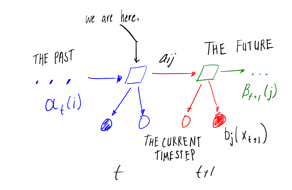
\[\xi_{t}(i, j) = \frac{\alpha_{t}(i)a_{ij}b_{j}(x_{t+1})\beta_{t+1}(j)}{P(O\vert\lambda)}\] where:

• \(\alpha_{t}(i)\) is the probability of observing symbols \(x_{1}, x_{2}, …, x_{t}\) and being in state i at time t, given \(\lambda\)
• \(a_{ij}\) is the probability of transitioning from state i to j
• \(b_{j}(x_{t+1})\) is the probability of observing symbol \(x_{t+1}\) in state j
• \(\beta_{t+1}(j)\) is the probability of starting in state \(i\) at time \(t\), and generating the rest of the sequence \(x_{t+1}, x_{t+2}, …, x_{T}\)
• \(P(O\vert\lambda)\) is the probability of observing the sequence given the model \(\lambda\)

which is equal to:

\[\xi_{t}(i,j) = \frac{\alpha_{t}(i)a_{ij}b_{j}(x_{t+1})\beta_{t+1}(j)}{\sum_{i=1}^N(\sum_{j=1}^N\alpha_{t}(i)a_{ij}b_{j}(x_{t+1})\beta_{t+1}(j))}\]

Visualizing this, we can see how the different probabilities fit together (the squares are hidden states, and the circles observation symbols):

When we translate this into code we have:

import numpy as np

def forward(x, A, B, pi, T, N):
	alpha  = np.zeros((T, N))
	alpha[0] = pi*B[:, x[0]]
	
	for i in range(1, T):
		alpha[i] = B[:, x[i]]*np.dot(alpha[i-1], A)	
	return alpha

def backward(X, A, B):
	beta = np.ones((X.shape[0], A.shape[0]))
	for t in range(X.shape[0]-2, -1, -1):
		beta[t] = np.sum((beta[t+1]*A)*B[:,X[t+1]], axis = 1).T
	return beta

def pr_transition(X, A, B, pi, N, T, t, i, j):
	return forward(X[:t+1], A, B, pi, t, N)[-1][i]*A[i,j]*B[j,X[t+1]]*backward(X[t+1:], A, B)[-1][j]


def pr_observation(X, A, B, pi, N, T, t):
	s = 0
	for j in range(N):
		s += np.sum((forward(X[:t+1], A, B, pi, t, N)[-1])*A[j,:]*B[j,X[t+1]]*backward(X[t+1:], A, B)[-1])
	return s	

A = np.array([[0.9, 0.1], [0.1, 0.9]])
B = np.array([[0.5, 0.5], [0.75, 0.25]])

pi = np.array([0.5, 0.5])
T = 3
N = 2

# O = [H, T]
x = np.array([0, 1, 1])

s = pr_observation(x, A, B, pi, N, T, 1)

print("P(O|model) = {}\n".format(s))

s0 = pr_transition(x, A, B, pi, N, T, 1, 0, 1)
s1 = pr_transition(x, A, B, pi, N, T, 1, 0, 0)
s2 = pr_transition(x, A, B, pi, N, T, 1, 1, 1)
s3 = pr_transition(x, A, B, pi, N, T, 1, 1, 0)


print("P(F, F | O, model) = {}".format(s1))
print("xi(t=2, F, F) = {}".format(s1/s))

print((s0+s1+s2+s3))

Output:

crazyeights@es-base:~$ python3 hmm_model.py 
P(O|model) = 0.22187500000000002

P(F, F | O, model) = 0.1125
xi(t=2, F, F) = 0.5070422535211268
0.221875

We can now use the functions above to calculate \(\xi_{t}(i,j)\):

def xi(X, A, B, pi, T, N, t, i, j):
	s = pr_observation(X, A, B, pi, N, T, t)
	s0 = pr_transition(X, A, B, pi, N, T, t, i, j)
	return s0/s

s = xi(x, A, B, pi, T, N, 1, 0, 0)

print("xi(t=2, F, F) = {}".format(s))

crazyeights@es-base:~$ python3 hmm_model.py 
xi(t=2, F, F) = 0.5070422535211268

Finally, we define \(\gamma_{t}(i)\) as the probability of being in state \(s_{i}\) at time t, given the observation sequence and the model, so if we sum \(\xi_{t}(i, j)\) over j we get: \(\gamma_{t}(i) = \sum_{j=1}^N\xi_{t}(i, j)\)

We can easily calculate that from what we have so far:

def gamma(X, A, B, pi, T, N, t, i):
	s = 0
	for j in range(N):
		s += xi(X, A, B, pi, T, N, t, i, j)
	return s

gamma(t=2, F) = 0.5352112676056338

That’s all for now folks! I will finish this someday…

Again apologies for any errors, I wrote this 3 months ago and never finished it.