Markov Chains and Hidden Markov Models
Markov models are very useful models that can describe many different processes. They are worth having some knowledge of. This post describes these models and their properties.
What is a Markov Model?
- A Markov model is a stochastic model used to model the changes of a system or process.
- A stochastic process describes a random variable that evolves over time. It describes behaviors a states and transitions, where transitions describe the probability of moving between states, and state refer to events (generally).
- These models are most commonly “discrete time” models, meaning that they consider the state of the system at distinct points in time. This includes things like player moves in a game, flips of a coin, steps in a random walk, and a pick of a ball from a bin.
Markov Property:
Markov models are based on the Markov property, that being that the future state is dependent only the on the current state.
- This means that the probability of transitioning to a subsequent state is only dependent on the current state, and not on how you reached the current state.
- This is expressed with conditional probabilities
- as if we are in state X, and we wish to know the probability of transitioning to state Y, we find \(P(Y \vert X)\).
Markov Chains:
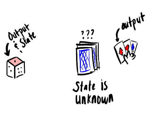
Markov chains are a type of Markov model, where the state of the system is fully observable, meaning that given the output we can determine the full state of the environment.
For example: flipping a fair coin or rolling a dice is a fully observable process, as we know the state of coin or dice (which face is up) by the output (heads or tails), whereas for modelling a deck of cards, selecting a card from the deck during a game of go-fish is not fully observable, as the card we recieve does not tell us the full state of the deck as it is dependent on the hands of other players.
The formal notation for this type of model is as follows:
- S - set of states
- T - set of transitions, where \(t_{i, j}\) is a transition between states i and j
- P - transition probability matrix, where \(p_{i, j}\) describes the probability of a transition between states i, and j
At each state a symbol is emitted, and over time the process generates a sequence of data.
When we model a sequence of events there is a definite beginning to the sequence, this should also be represented in our model:
- \(I\) is the vector of probabilities, where \(I_{j}, j \in S\) is the probability that state j is the initial state.
Example:
The most basic example of such a model is a model of a coin:
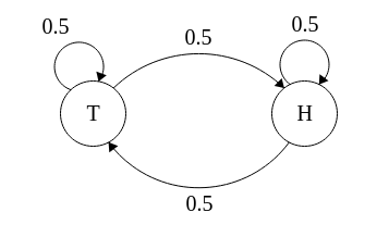
With states \(S = \{H, T\}\), which is the side of the coin facing up. At each state either heads (H), or tails (T) is emitted.
In this model transitions from H to H, H to T, T to T, and T to H are possible, and each transition would have an equal probability of 0.5. We represent these probabilities with the following matrix P, shown as a table for visual clarity.
| H | T | |
|---|---|---|
| H | 0.5 | 0.5 |
| T | 0.5 | 0.5 |
It would also have equal initial probabilities \(I = \{0.5, 0.5\}\), as the probability of a particular coin toss being heads or tails is equal, so the coin could be in either state initially with equal probability.
We can visualize this model as:
The probability of a particular transition occurring at the current state, without considering any past state is:
Let \(X_{t}\) be the state of the process at time t (after t coin flips), then the probability of being in state i at time t+1 is: \[P(X_{t+1}=i | X_{t}=j) = P_{ji} = 0.5 \] where \(P_{ji}\) is the corresponding entry in the probability matrix.
With our model we can now calculate the probability of a particular sequence of events (or states) occuring. We can write this sequence as \(X = \{x_{1}, x_{2}, x_{3}, … x_{T}\}\), where T is the length of the sequence (the number of steps or actions) and \(x_{i}\) is the state at time i This is calculated as: \[P(X) = P(x_{1})P(x_{2} | x_{1})P(x_{3}|x_{2})…P(x_{T} | x_{T-1})\] or: \[P(X) = P(x_{1})\prod_{i=1}^{T-1}P(x_{i+1} | x_{i})\]
For example for a sequence \(X = \{H, T, T, H\}\), we have:
\[P(X) = P(x_{1} = T)P(x_{2} = T | x_{1} = H)P(x_{3} = T | x_{2} = T)P(x_{4} = H | x_{3} = T)\] \[P(X) = (0.5)(0.5)(0.5)(0.5)(0.5) = 0.0625 \]
Because this is a fair coin, all sequences that are the same length are equally likely.
The most important thing to note about this kind of model is that the current state is most often equal to the symbol emitted for that for that state.
Hidden Markov Models:
A Hidden Markov Model (HMM) is a type of Markov model that has hidden states, as well as observation symbols. Each hidden state emits a symbol with a particular probability, and transitions between hidden states occur with a particular probability.
This is because the Markov model underlying the data that is being modeled is hidden or unknown, so that at any time that state of a system is only partially observable. This means that we can not determine the complete state of the system from its output. We may only know the observation data (ie. sequences of output symbols) and not information about the states.
Example:
Here is an example to better explain these concepts:
This example is very common used, it is called the fair-bet casino.
- The game involves flipping a coin
- The dealer may switch between a fair and biased coin
- The player doesn’t know which coin they are currently flipping
- The probability of the player getting a particular outcome is dependent on which coin is being flipped.
- The game basically produces a sequence of coin flips.
Here is a sketch to illustrate the problem, in which F is the fair coin, B is the biased coin, and H is heads, T is tails.
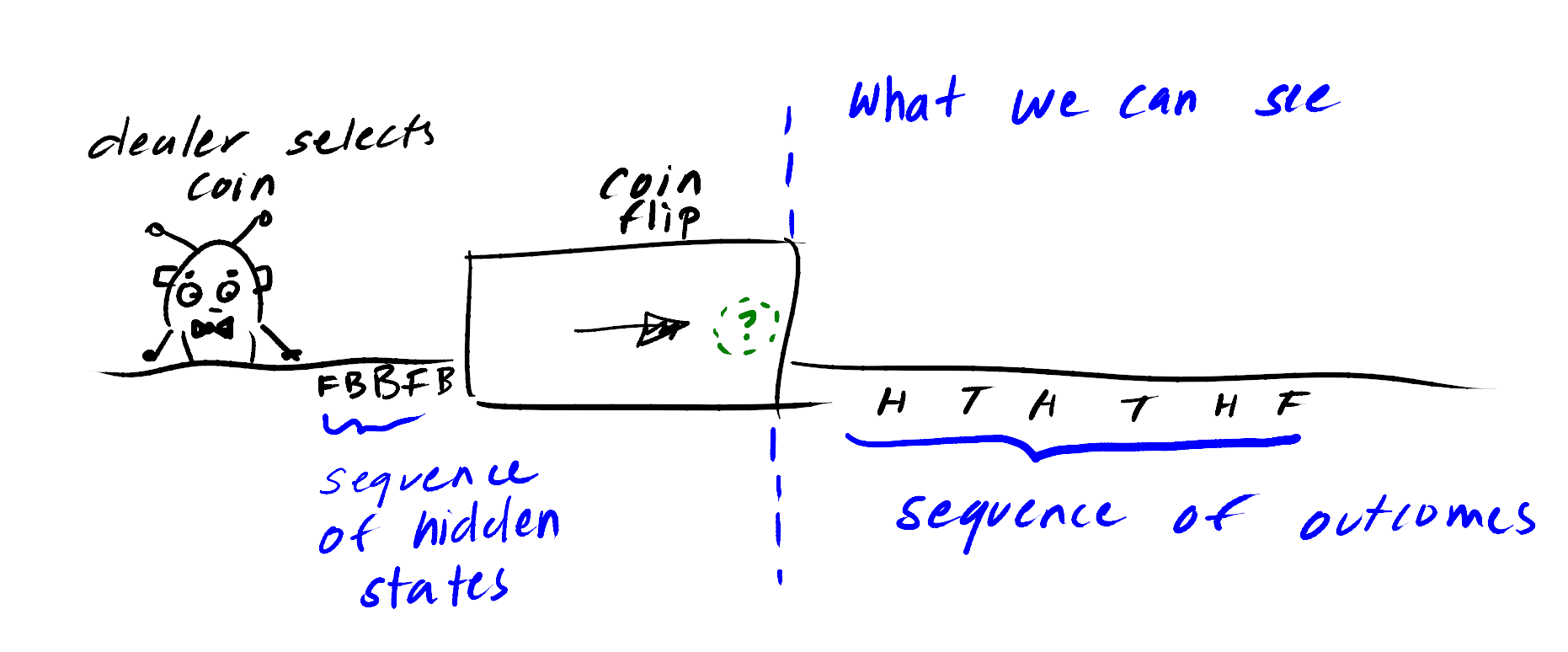
The green circle symbolizes the current coin flip. Regardless of the outcome we will only be able to estimate which coin was flipped to produce it. We call this unknown the hidden state.
This can be represented with the following model:
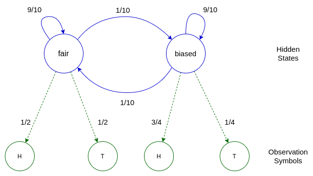
In the above model the transitions between hidden states are shown in blue, at each time step we emit a symbol shown in green.
Notation:
A Hidden Markov Model has the following notation:
- N - number of states
- M - number of observation symbols
- S - set of hidden states
- \(V\) is the set of observation symbols \(V = \{v_{0}, v_{1}, …, v_{M}\}\)
- \(\Pi\) is the set of probabilities that each state is the initial state, or \(\pi_{i} = P(S_{t} = i)\), or the probability of being in state i, at time t=1
- A - the transition probability matrix, where an entry \(a_{ij}\) is the probability of transitioning from state i to state j
- B - the emission probability matrix, where an entry \(b_{j}(k)\) is the probability of observing symbol \(v_{k}\) in state j
Back to the fair-bet casino example, we would have the following model (Note I am using the same probabilities as in the diagram above):
- There are two hidden states, and 2 observation symbols: N = 2, M = 2
- The hidden states describe which coin is currently being flipped, as which coin that is being flipped will greately effect the probability of getting a particular outcome. These hidden states are \(S = {F, B}\), where F represents the fair coin, and B represents the biased coin.
- We see either heads or tails when we flip the coin, so \(V = {H, T}\)
- We can say each of the hidden states can be the initial state with equal probability: \(\Pi = \{0.5, 0.5\}\)
- We have the following transition probability matrix:
-
A =
F B F 0.9 0.1 B 0.1 0.9 - We have the following emission matrix:
-
B =
H T F 0.5 0.5 B 0.75 0.25
Now that we have our model, what do we use it for?
We can use the hidden markov model (HMM) to solve 4 fundamental problems:
- Decoding problems For a particular model, and observation sequence, estimate the most likely (hidden) state sequence.
- Evaluation problems Given a model, and an observation, find the probability of the observation sequence occurs under the given model. This process involves a maximum likelihood estimates of the attributes sometimes called an evaluation problems.
- Training problems Given a set of observation sequences, compute a model that best explains the sequences.
Here we will focus on evaluation problems.
Probability of Seeing a Particular Observation Sequence:
The basis of the evaluation problem is the ability to calculate probability of a observation sequence occuring, given a particular state sequence and model.
The probability of being in a particular state, when t=1 (the inital state) is \(P(s_{i}) = \pi_{i}\).
For every subsequent state the probability is dependent on the previous state \(P(s_{i} \vert s_{i-1})\) For example: in the Fair-Bet Casino, for a transition F to B, we have: \(P(F \vert B) = 0.1\), which is \(a_{F,B}\) in our transmission matrix A.
The probability of seeing a particular observation symbol is dependent on the current state. For symbol \(v_{k}\) and the current state i, \(P(v_{k} \vert i)\) For Example: in the Fair-Bet Casino, for the hidden state, observation symbol pair B, T we have \(P(T \vert B) = 0.25\), which is \(b_{1, 1}\) (1,1 is the index of B, T in matrix B) in the emission matrix B.
We can calculate the probability of observation sequence, given a particular set of hidden states for a particular model \(\lambda\). For a sequence of observation symbols \(X = \{x_{1}, x_{2}, …, x_{T}\}\), and sequence of hidden states \(S = \{s_{1}, s_{2}, .., s_{T}\}\), we have:
\[P(X, S \vert \lambda) = P(S \vert \lambda)P(X \vert S)\]
which is equal to:
\[P(X, S \vert \lambda) = P(s_{1})P(x_{1} \vert s_{1})P(s_{2} \vert s_{1})P(x_{2} \vert s_{2})\]
\[…P(s_{T} \vert s_{T-1})P(x_{T} \vert s_{T})\]
This can be written more clearly as:
\[P(X, S\vert \lambda) = P(s_{1})P(x_{1} \vert s_{1})\prod_{i=2}^{T}P(s_{i} \vert s_{i-1})P(x_{i} \vert s_{i})\]
or
\[P(X, S \vert \lambda) = \pi_{i}\prod_{i=2}^{T}P(s_{i} \vert s_{i-1})\prod_{i=1}^{T}P(x_{i} \vert s_{i})\]
Or even better, using our matrices:
- \(S_{t}\) denotes the state at time t
- \(a_{ij}\) denotes the transition probability from states i to j, at time t: \(a_{ij} = P(S_{t} = j \vert S_{t-1} = i)\)
- \(b_{j}(v_{k})\) denotes the probability of observing symbol (\v_{k}\) in state j, at time t: \(b_{j}(v_{k}) = P(X_{t} = v_{k} \vert S_{t} = j)\)
Putting this together we get:
\[P(X, S \vert \lambda) = \pi_{i}b_{i, t=1}(v_{k})\prod_{t=2}^{T} b_{j}(v_{k})a_{ij}\]
Note: \(b_{j}(v_{k})\) for t=1 is written as \(b_{i, t=1}(v_{k})\) to avoid confusion.
Example: Back to the Fair-Bet Casino
Let’s say we have observation sequence \(X = \{H, T, H, H\}\), and hidden states \(S = \{F, B, B, B\}\), we calculate the probability that this occurs in our model \(\lambda\) as: \[P(X, S \vert \lambda) = P(F)P(H \vert F)P(B \vert F)P(T \vert B)P(B \vert B)P(H \vert B)P(B \vert B)P(H \vert B)\] \[= (0.5)(0.5)(0.1)(0.25)(0.9)(0.75)(0.9)(0.75)(0.9)\] \[= 2.56 \times 10^{-3} \]
Back to the evaluation problem.
The evaluation problem is the problem of finding the probability that a particular observation occurs occurs in a model. We no longer have a hidden state sequence to base this probability on. This is where the forward algorithm comes in.
Forward Algorithm:
The forward algorithm calculates the probability of being in the t-th time step, and having seen observations \(X = \{x_{1}, x_{2}, …, x_{t}\}\) for a model \(\lambda\).
This can be formulated as follows:
The probability of observing a sequence \(X = x_{1},…,x_{T}\) of length T is given by: \[P(X) = \sum_{S}P(X \vert S)P(S)\]
where the sum is over all possible hidden state sequences \(S = s_{1}, …, S_{T}\). This can be found using the forward algorithm.
Forward Probability
The Forward Probability is the probability of seeing the observations \(x_{1}, x_{2},…,x_{t}\) and being in state i at time t, given a model \(\lambda = \{A, B, \pi\}\).
It uses the computed probability at the current time step to derive the probability of being in a particular hidden state at the next time step.
The forward algorithm calculates this forward probability for all hidden states.
This is found recursively: \[\alpha_{i}(1) = \pi_{i}b_{i}(x_{1})\] \[\alpha_{i}(t+1) = b_{i}(x_{t+1})\sum_{j=1}^N \alpha_{j}(t)a_{ji}\]
where:
- \(\alpha_{i}(t)\) is the probability of being in state i at time t. This is the value that is returned.
- \(\pi_{i}\) is the probability that the initial state is s
- \(b_{i}(x_{t})\) is the probability of seeing symbol \(x_{t}\) in state i
- \(a_{ij}\) is the probability of being in state i given the previous state was state j
Example: For example for the Fair-Bet Casino, we can find the probability that a particular observation sequence occurs. For the observation sequence: \(X = \{H, T, T\}\), we have the following possible sequences of hidden states (F for fair coin, B for biased coin):
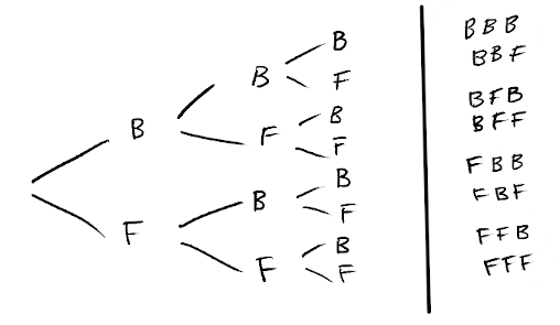
which will produce the following probabilities when we calculate \(P(X, S \vert \lambda)\) for each hidden state sequence individually:
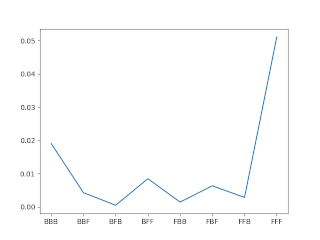
We can use the forward algorithm to calculate the probability of this sequence occuring for all possible sequence of hidden states.
Note: the multiplication of \(\alpha(i)\) and A seen below is the dot product
For the initial state:
When \(t = 1\), the observation symbol is \(x_{1} = H\)
We have the following:
\[\alpha_{i}(1) = \pi_{1}b_{i}(x_{1}), i \in \{F, B\}, x_{1} = H\]
We can vectorize this calculation so we can calculate the probabilities for all states at the same time.
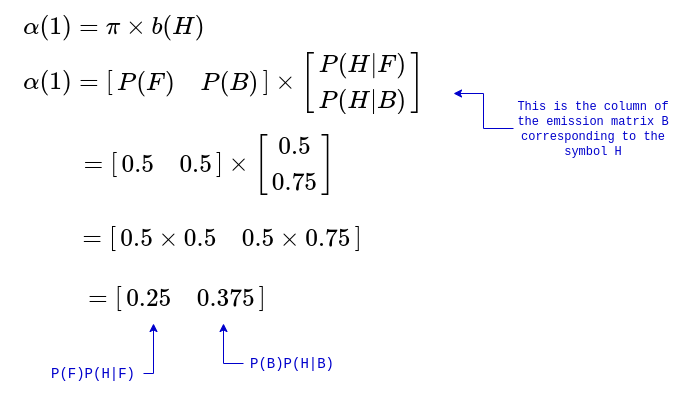
For t=2:
When \(t = 2\), the observation symbol is \(x_{2} = T\)
We have the following:
\[\alpha_{i}(2) = b(T)\times(\sum_{j}^{S = \{F, B\}}\alpha_{i}(1)a_{ij})\]
We have the following, using the previously calculated \(\alpha(1)\):
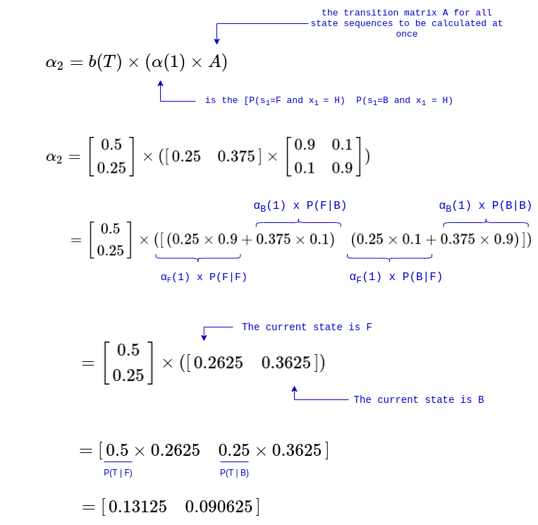
For t=3:
When \(t = 3\), the observation symbol is \(x_{3} = T\)
We have the following, using the previously calculated \(\alpha(2)\):
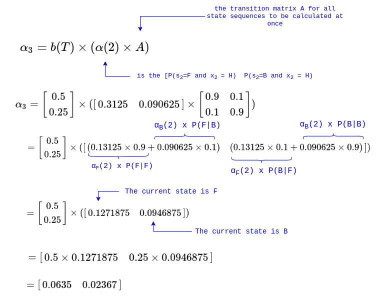
We now take the sum of the final probability of both the final states: \[P(X \vert \lambda) = \sum \alpha(3) = 0.0635 + 0.02367 = 0.08717\]
This is equal (the one that was calculated manually was rounded to 4-5 decimal places, so it is off by ~0.001), to the probability found by computing the probability of every possible state sequence seperately and getting the sum (as seen in the figure showing the probability distribution above). It is more efficient however. Here it is in python, using the same example, and a for loop to loop through each time step:
import numpy as np

def forward(x, A, B, pi, T, N):
	alpha  = np.zeros((T, N))
	alpha[0] = pi*B[:, x[0]]

	for i in range(1, T):
		alpha[i] = B[:, x[i]]*np.dot(alpha[i-1], A)

	return alpha

A = np.array([[0.9, 0.1], [0.1, 0.9]])
B = np.array([[0.5, 0.5], [0.75, 0.25]])

pi = np.array([0.5, 0.5])
T = 3
N = 2

# O = [H, T]
x = np.array([0, 1, 1])

alpha = forward(x, A, B, pi, T, N)
# The final probability:
print(np.sum(alpha[2]))
Running it gives us:
crazyeights@es-base:~$ python3 forward.py
0.087265625
The forward algorithm is one of the fundamental building blocks of many other algorithms that use this probabilistic model.
These types of models have applications in fields such as bioinformatics, and ML. There are applications in computing for intrusion detection and verification are particularly intresting.
In the future I hope to write about these, as well as the other types of problems the HMM can solve, such as learning problems, sequence alignment, etc.
(Sorry for any human error 😓)